Predictive model comparison

Below is a portion of one of the projects I completed for my graduate degree. The task was to build and test three predictive models on the same dataset to see which was able to predict Emergency Department Overcrowding.

Predictive model comparison with Emergency department data

This code will use R to explore the predictive qualities of Support Vector Machine (SVM), Naive Bayes, and Random Forest in relation to emergency department overcrowding.

Data file (this was cleaned and brought into R)

project-predictive-data-final Download

File (Header) Key

Packages

install.packages("tidyverse")
install.packages("descr")
install.packages("forcats")
install.packages("e1071")
install.packages("caret")
install.packages("lattice")
install.packages("caTools")
install.packages("rmarkdown")
install.packages("ggplot2")
install.packages("corrplot")
install.packages("randomForest")
install.packages("plyr")
install.packages("ROSE")
install.packages("readxl")
install.packages("lubridate")
install.packages("zoo")
install.packages("magrittr")
install.packages("ROCR")
install.packages("pROC")
install.packages("readr")

library(plyr)
library(dplyr)
library(tidyverse)
library(descr) # Descriptive Statistics
library(ggplot2)
library(forcats) # Tools for Working with Categorical Variables (Factors) 
library(e1071) # Misc Functions of the Department of Statistics, Probability Theory Group
library(lattice)
library(caret) # Classification and Regression Training
library(caTools)
library(rmarkdown)
library(ggplot2)
library(corrplot)
library(randomForest)


library(ROSE)
library(readxl)
library(lubridate)
library(zoo)
library(magrittr)
library(ROCR)
library(pROC)
library(readr)

Load file – reload the same file

nedoc_data <- read.csv(file.choose())
dfilter1 <- read.csv(file.choose())
Pdfilter1 <- read.csv(file.choose())


#PD filter is for predictive
#D filter is for general analysis and exploratory predictive

Data Prep

#####-----------------------DATA PREP

dfilter1$OVR <- as.factor(dfilter1$OVR)
dfilter1$SEV <- as.factor(dfilter1$SEV)
dfilter1$DNG <- as.factor(dfilter1$DNG)
dfilter1$Hour <- as.factor(dfilter1$Hour)
dfilter1$Day <- as.factor(dfilter1$Day)
dfilter1$Week <- as.factor(dfilter1$Week)


DNGfile <- filter(dfilter1, dfilter1$NAVG == 4)
SEVfile <- filter(dfilter1, dfilter1$NAVG == 3)
OVRfile <- filter(dfilter1, dfilter1$NAVG == 2)

NE_Week <- filter(dfilter1, dfilter1$BSY == 1, dfilter1$DNG == 0, dfilter1$Week %in% c(2,3,4))
NE_Week2 <- filter(dfilter1, dfilter1$DNG == 0, dfilter1$Week %in% c(1,2,3,4))

#Can use regular filter file because after clean I move data into different files for pred
#move OVR to front with Date so that you can have both Naive and SVM with same dataset


Pdfilter1$OVR <- as.factor(Pdfilter1$OVR)
Pdfilter1$Hour <- as.factor(Pdfilter1$Hour)
Pdfilter1$Day <- as.factor(Pdfilter1$Day)
Pdfilter1$Week <- as.factor(Pdfilter1$Week)

Pdfilter1$OVRcut <- ifelse(Pdfilter1$OVR == 0,"good","bad")
Pdfilter1$OVRcut <- as.factor(Pdfilter1$OVRcut)
summary(Pdfilter1$DEP)
Pdfilter1$DEPcut <- cut(Pdfilter1$DEP, breaks=c(20,43,76,109),
                      labels=c("bottom 25%","middle 50%", "top 25%"))
table(Pdfilter1$DEPcut)
summary(Pdfilter1$EDW)
Pdfilter1$EDWcut <- cut(Pdfilter1$EDW, breaks=c(0,6,14,29),
                      labels=c("bottom 25%","middle 50%", "top 25%"))
table(Pdfilter1$EDWcut)
summary(Pdfilter1$CC)
Pdfilter1$CCcut <- cut(Pdfilter1$CC, breaks=c(0,3.5,7,14),
                     labels=c("bottom 25%","middle 50%", "top 25%"))
table(Pdfilter1$CCcut)
summary(Pdfilter1$DTB)
Pdfilter1$DTBcut <- cut(Pdfilter1$DTB, breaks=c(-0.07,0.03,0.8825,6.76),
                      labels=c("bottom 25%","middle 50%", "top 25%"))
table(Pdfilter1$DTBcut)
summary(Pdfilter1$LAT)
Pdfilter1$LAT2 <- Pdfilter1$LAT
Pdfilter1$LAT2[Pdfilter1$LAT2 == 0.00] <- 0.01
Pdfilter1$LATcut <- cut(Pdfilter1$LAT2, breaks=c(0.00,1.63,6.562,30.02),
                      labels=c("bottom 25%","middle 50%", "top 25%"))
table(Pdfilter1$LATcut)

str(Pdfilter1)

SVMD1 <- Pdfilter1

SVMD1$OVR <- as.factor(SVMD$OVR)
SVMD1$Hour <- as.factor(SVMD$Hour)
SVMD1$Day <- as.factor(SVMD$Day)
SVMD1$Week <- as.factor(SVMD$Week)

NaiveD1 <- Pdfilter1
str(NaiveD1)
NaiveD1$OVRcut <- ifelse(NaiveD1$OVR == 0,"good","bad")
NaiveD1$OVRcut <- as.factor(NaiveD1$OVRcut)
summary(NaiveD1$DEP)
NaiveD1$DEPcut <- cut(NaiveD1$DEP, breaks=c(20,43,76,109),
                   labels=c("bottom 25%","middle 50%", "top 25%"))
table(NaiveD1$DEPcut)
summary(NaiveD1$EDW)
NaiveD1$EDWcut <- cut(NaiveD1$EDW, breaks=c(0,6,14,29),
                      labels=c("bottom 25%","middle 50%", "top 25%"))
table(NaiveD1$EDWcut)
summary(NaiveD1$CC)
NaiveD1$CCcut <- cut(NaiveD1$CC, breaks=c(0,3.5,7,14),
                      labels=c("bottom 25%","middle 50%", "top 25%"))
table(NaiveD1$CCcut)
summary(NaiveD1$DTB)
NaiveD1$DTBcut <- cut(NaiveD1$DTB, breaks=c(-0.07,0.03,0.8825,6.76),
                      labels=c("bottom 25%","middle 50%", "top 25%"))
table(NaiveD1$DTBcut)
summary(NaiveD1$LAT)
NaiveD1$LATcut <- cut(NaiveD1$LAT, breaks=c(0.0,1.63,6.562,30.02),
                      labels=c("bottom 25%","middle 50%", "top 25%"))
table(NaiveD1$LATcut)

SVMData <- select(SVMD1, DEP, EDW, CC, DTB, LAT, Hour, Day, Week, OVR)
NaiveData <- select(NaiveD1,OVRcut, DEPcut,EDWcut,CCcut,DTBcut,LATcut,Hour, Day, Week)

Data Viz pre-predictive

#############------------------DATA VIZ


#Distribution of NeDoc Scores
DViz <- ggplot(data=dfilter1, aes(x=AVG)) + 
  geom_histogram(aes(y=..density..),
                 col='black', 
                 fill='dodgerblue1', 
                 alpha=0.3) +
  geom_density(adjust=3)
print(DViz + theme(plot.title=element_text(face="bold")) + ggtitle('Distribution of the NeDoc Averages'))

#NE_Week2 Data viz of distribution Shows more balanced avg without week 5 or Danger (only in week 1)
DVizNE <- ggplot(data=NE_Week2, aes(x=AVG)) + 
  geom_histogram(aes(y=..density..),
                 col='black', 
                 fill='dodgerblue1', 
                 alpha=0.3) +
  geom_density(adjust=3)
print(DVizNE + theme(plot.title=element_text(face="bold")) + ggtitle('NE_Week Distribution of the NeDoc Averages'))

##hR CHART SHOWS GOOD REP FOR OVR
NAVGdist <- ggplot(data=dfilter1, aes(x=dfilter1$Hour, fill=OVR)) + 
  geom_bar(aes(y = (..count..)/sum(..count..)), position='stack', alpha=0.5) + scale_y_continuous(labels=scales::percent)
print(NAVGdist + theme(plot.title=element_text(face="bold")) + ggtitle('Hour to Overcrowded'))

##Pretty cool Day Chart
NAVGdist <- ggplot(data=dfilter1, aes(x=dfilter1$Day, fill=OVR)) + 
  geom_bar(aes(y = (..count..)/sum(..count..)), position='stack', alpha=0.5) + scale_y_continuous(labels=scales::percent)
print(NAVGdist + theme(plot.title=element_text(face="bold")) + ggtitle('Day to Overcrowded'))

#good rep of decline in overcrowded
NAVGdist <- ggplot(data=dfilter1, aes(x=dfilter1$Week, fill=OVR)) + 
  geom_bar(aes(y = (..count..)/sum(..count..)), position='stack', alpha=0.5) + scale_y_continuous(labels=scales::percent)
print(NAVGdist + theme(plot.title=element_text(face="bold")) + ggtitle('Week to Overcrowded'))


#Dep Higher More OVR, cc, LAT  (EDW, DTB even distribution)  
#Dont know which charts to use but here is the build just need to change the name
NAVGdist <- ggplot(data=dfilter1, aes(x=dfilter1$Week, fill=OVR)) + 
  geom_bar(aes(y = (..count..)/sum(..count..)), position='stack', alpha=0.5) + scale_y_continuous(labels=scales::percent)
print(NAVGdist + theme(plot.title=element_text(face="bold")) + ggtitle('Home Ownership vs Loan Default'))

Establishing train and test datasets to be used through different models

#########------------------PREDICTIVE
#Establish train and test models
##I think I can have 1 full file and identify different test pieces below


Predictivedata <- Pdfilter1
set.seed(101)

PredData <- sample.split(Predictivedata$OVR, SplitRatio = 0.7)
PredDatatrain <- subset(Predictivedata, PredData == TRUE)
PredDatatest <- subset(Predictivedata, PredData == FALSE)

AASVMDatatrain <- select(PredDatatrain, DEP, EDW, CC, DTB, LAT, Hour, Day, Week, OVR)
AASVMDatatest <- select(PredDatatest, DEP, EDW, CC, DTB, LAT, Hour, Day, Week, OVR)
AANaiveDatatrain <- select(PredDatatrain,OVRcut, DEPcut,EDWcut,CCcut,DTBcut,LATcut,Hour, Day, Week)
AANaiveDatatest <- select(PredDatatest,OVRcut, DEPcut,EDWcut,CCcut,DTBcut,LATcut,Hour, Day, Week)
AARTDatatrain <- select(PredDatatrain, DEP, EDW, CC, DTB, LAT, Hour, Day, Week, OVR)
AARTDatatest <- select(PredDatatest, DEP, EDW, CC, DTB, LAT, Hour, Day, Week, OVR)

SVM

##SVM
str(AASVMDatatrain)

SVMmodelA <- svm(AASVMDatatrain$OVR ~., data = AASVMDatatrain[1:9])
summary(SVMmodelA)

SVMpreds <- predict(SVMmodelA,AASVMDatatest[1:8])
table(SVMpreds, AASVMDatatest$OVR)

SVMpreds.tuned <-svm(AASVMDatatrain$OVR ~., data = AASVMDatatrain[1:9], kernal='radial', cost =70, gamma=0.2)
SVMpreds2 <- predict(SVMpreds.tuned, AASVMDatatest[1:8])
confusionMatrix(SVMpreds2, AASVMDatatest$OVR)

#need to create a fake one with OVR reversed for ROC chart
SVMROCtrain <- AASVMDatatrain
SVMROCtrain$ROVR <- ifelse(SVMROCtrain$OVR %in% c(1), 0, 1)
SVMROCtest <- AASVMDatatest
SVMROCtest$ROVR <- ifelse(SVMROCtest$OVR %in% c(1), 0, 1)

SVMROCtrain$ROVR <- as.factor(SVMROCtrain$ROVR)
SVMROCtest$ROVR <- as.factor(SVMROCtest$ROVR)

SVMmodelROC <-svm(SVMROCtrain$ROVR ~., data = SVMROCtrain[1:10], kernal='radial', cost =70, gamma=0.2)
SVMpredsROC <- predict(SVMmodelROC, SVMROCtest[1:9])
confusionMatrix(SVMpredsROC, SVMROCtest$ROVR)

Naive Bayes

## Naive
AANaiveDatatrain
Naiveclassy <- naiveBayes(OVRcut ~ DEPcut+EDWcut+CCcut+DTBcut+LATcut+Hour+Day+Week,AANaiveDatatrain)
Naiveclassy

Naivepreds <- predict(Naiveclassy, select(AANaiveDatatest, DEPcut,EDWcut,CCcut,DTBcut,LATcut,Hour, Day, Week), type="raw")
summary(Naivepreds)

AANaiveDatatest$Naive_preds <- ifelse(Naivepreds[,"good"] > 0.70, "good", "bad")
table(AANaiveDatatest$Naive_preds)

NaiveAtestA<-factor(AANaiveDatatest$OVRcut)
NaiveAtestB<-factor(AANaiveDatatest$Naive_preds)
confusionMatrix(NaiveAtestB, NaiveAtestA)

Logistic Regression

##Logistic Regression
AARTDatatrain
AARTDatatest$OVR

logisticreg <- glm(OVR~., family=binomial(link='logit'), data = AARTDatatrain)
LRpreds <- predict(logisticreg,AARTDatatest, type ='response')
LRpreds <- ifelse(LRpreds > 0.5,1,0)
compare <- data.frame(actual = AARTDatatest$OVR, predicted = LRpreds)
misClasificError <- mean(LRpreds != AARTDatatest$OVR)
print(paste('Accuracy',1-misClasificError))

confusionMatrix(as.factor(LRpreds),as.factor(AARTDatatest$OVR))

Random Forest

##Random Forest
AARTDatatrain

RFmodel <- randomForest(OVR ~ ., data=AARTDatatrain, importance = TRUE, ntree = 200, na.action = na.omit)
RFpreds <- predict(RFmodel, AARTDatatest, type='class')
RFoutput <- confusionMatrix(AARTDatatest$OVR, RFpreds)
paste0(RFoutput$overall[1])
#Confusion Matrix
RFoutput

Here is each models confusion matrix

#SVM
SVMROCtrain$ROVR <- as.factor(SVMROCtrain$ROVR)
SVMROCtest$ROVR <- as.factor(SVMROCtest$ROVR)

SVMmodelROC <-svm(SVMROCtrain$ROVR ~., data = SVMROCtrain[1:10], kernal='radial', cost =70, gamma=0.2)
SVMpredsROC <- predict(SVMmodelROC, SVMROCtest[1:9])
confusionMatrix(SVMpredsROC, SVMROCtest$ROVR)

#Naive Bayes
NaiveAtestA<-factor(AANaiveDatatest$OVRcut)
NaiveAtestB<-factor(AANaiveDatatest$Naive_preds)
confusionMatrix(NaiveAtestB, NaiveAtestA)

#Logistic Regression
confusionMatrix(as.factor(LRpreds),as.factor(AARTDatatest$OVR))

#Random Forest
RFoutput <- confusionMatrix(AARTDatatest$OVR, RFpreds)
RFoutput

ROC Curve

##Full comparison ROC Curve
#ROC Linear Regression
LRval <- as.numeric(paste0(LRpreds))
LRpredObj <- prediction(LRval,AARTDatatest$OVR)
LRrocObj <- performance(LRpredObj, measure="tpr", x.measure="fpr") 
LRaucObj <- performance(LRpredObj, measure="auc")


#ROC Random Forest
predRFprob <- predict(RFmodel, AARTDatatest, type = "prob")
RFval <- as.numeric(paste0(predRFprob[,2]))
RFpredObj <- prediction(RFval, AARTDatatest$OVR)
RFrocObj <- performance(RFpredObj, measure="tpr", x.measure="fpr") 
RFaucObj <- performance(RFpredObj, measure="auc")


#ROC Naive Bayes
predNBprob <- predict(Naiveclassy, AANaiveDatatest, type = "prob")
NBval <- as.numeric(paste0(Naivepreds[,2]))
NBpredObj <- prediction(NBval,AANaiveDatatest$OVR)
NBrocObj <- performance(LRpredObj, measure="tpr", x.measure="fpr") 
NBaucObj <- performance(LRpredObj, measure="auc")

#ROC SVM
##Keep working on it for SVM

SVMmodelROC <-svm(SVMROCtrain$ROVR ~., data = SVMROCtrain[1:10], kernal='radial', cost =70, gamma=0.2)
SVMpredsROC <- predict(SVMmodelROC, SVMROCtest[1:9])

SVMrocObj <- roc(response = SVMROCtest$ROVR, predictor =as.numeric(SVMpredsROC))



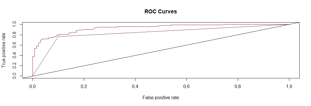
plot(LRrocObj, col = "blue", lwd = 1, main = "ROC Curves")
plot(RFrocObj, add = TRUE, col = "red")
#plot(SVMrocObj, add = TRUE, col = "green")
plot(NBrocObj, add = TRUE, col = "brown")
abline(a=0, b=1)

(NB) Naive Bayes and (LR) logistic regression have the exact same line (it appears brown but both the brown and blue lines are the same).

This comparison model shows that with this data in relation to emergency department overcrowding the Random Forest model was the best at predicting ED overcrowding.